In this article, we demonstrate how to extend C++ code to SYCL* code and actively leverage your GPU. These examples will show how you can take advantage of different SYCL kernels and memory management techniques. You will see how to achieve great gains in performance by only investing limited coding effort.
- We use the Intel® oneAPI DPC++/C++ Compiler to compile both the C++ and SYCL code.
- Intel® VTune™ Profiler will be used to analyze performance metrics of different SYCL kernel and memory management techniques. Applying performance analysis this way, we will verify our progress of improving performance through SYCL-based parallel code execution on a GPU.
Let’s first introduce the basic setup and then walk through the steps of applying improvements by adding SYCL kernels:
Setup
The following hardware and software configuration is used to gather the VTune Profiler performance analysis data used throughout the article:
- Application: A simple 2d-matrix operation:
#include<iostream> const int N = 8192; const int M = 8192; int main(){ int* array[N]; for (int i = 0; i < N; i++) array[i] = (int*)malloc(M * sizeof(int)); for(int i = 0; i < N; i++){ for(int j = 0; j < M; j++){ array[i][j]=i*j; } } return 0; } - Tools:
- Intel oneAPI DPC++/C++ Compiler 2023.0
- Intel VTune Profiler 2023.0
- CPU/GPU:
- 11th Gen Intel® Core™ Processor i9-11900KB @ 3.30GHz 3.0 with
- Intel® Iris® Xe Graphics GT2 (arch=Xe; former code name=Tiger Lake)
- Operating System: Ubuntu* 20.04.4
Turn on SYCL Compiler Support
To enable C++ SYCL language extension with the compiler, all we need is the addition of the -fsycl option:
icpx -fsycl -O3 -std=c++17 main.cpp -o matrix
What Is a SYCL Kernel Anyway?
A kernel is an abstract concept to express parallelism and leverage the hardware resources of the target device. A SYCL kernel creates multiple instances of a single operation that will run simultaneously.
Depending on the type of problem, kernels can be one-, two-, or three-dimensional. There are different forms of SYCL kernels that follow different syntax and support different features. Some forms of kernels are more suitable for some scenarios than others.
Kernels are submitted to a device queue for execution. A queue is directly mapped to a specific device. Therefore, kernels submitted to a device queue are executed by a certain target device.
Now let us look at different types of SYCL kernels and how we can add them to C++ code.
Types of SYCL Kernels
There are various types of parallel kernels that can be suitable and easily expressible for different algorithms. In our example, we will show how one such algorithm can be transformed using 3 different types of kernels. You can then apply similar thought processes to decide which kernel implementation or combinations of kernels to choose for your own application based on your requirements.
1. Basic Parallel Kernel
This type of kernel is easy to implement but usually only suitable for algorithms that rely on very straightforward data parallelism.
The first parameter of the template function (parallel_for) is the range. The range can be of 1, 2, or 3 dimensions. Instances of the range class are used to describe the execution ranges of a kernel function.
The second parameter, id class, represents a container that has the capacity of 1, 2, or 3 integers. One alternative for the id class is to use the item class which provides the programmer with more control for queries. It is an encapsulation of the execution range of the kernel and the instance’s index within that range. Thus, it helps the programmer count the linearized index without requiring an additional argument.
In this example, we replace the outer loop with the parallel_for function and other necessary parameters:
Before:
device_queue.submit([&](handler &h){
    auto buffer_accessor_device=
    buff.get_access<access::mode::read_write>(h);
    for(int i=0;i<N;j++)
        for(int j=0;j<M;j++)
		    array[i][j] = i*j;
});
After:
device_queue.submit([&](handler &h){
    auto buffer_accessor_device=buff.get_access<access::mode::read_write>(h);
    h.parallel_for<class multiplication>(range<1>(N),[=](id<1> i){
    	for(int j=0;j<M;j++)
      	    buffer_accessor_device[i][j] = i*j;
    });
});
Alternatively, we can also eliminate the inner loop and introduce a 2d range and 2d id class:
device_queue.submit([&](handler &h){
    auto buffer_accessor_device=buff.get_access<access::mode::read_write>(h);
    h.parallel_for<class multiplication>(range<2>(N,M),[=](id<2> idx){
        int i=idx[0];
        int j=idx[1];
        buffer_accessor_device[i][j] = i*j;
    });
});
The second approach provides a cleaner way to express the parallelism of a nested loop using the Basic Parallel Kernel.
VTune Profiler allows us to conduct an analysis of the different performance metrics for this implementation. Using GPU Compute/Media Hotspots analysis we can understand the utilization of different hardware units of GPU.
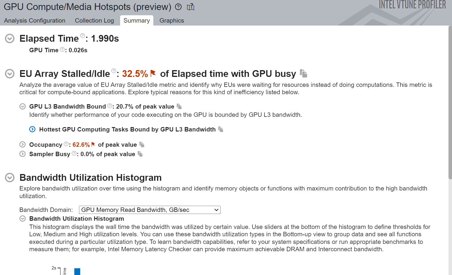
Figure 1. Summary view of Basic Parallel Kernel Implementation
Figure 1 shows that the execution unit (EU) Array Stalled/Idle time is 32.5% and it has been marked red which means there are some opportunities for optimization. VTune Profiler also reports that the reason for this inefficiency is because the application is bounded by GPU L3 cache bandwidth.
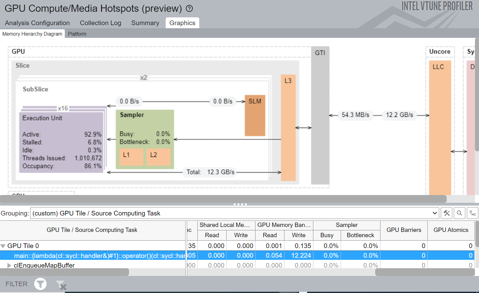
Figure 2. Memory Hierarchy Diagram of Basic Parallel Kernel Implementation
In Figure 2, we have a closer look at the Memory Hierarchy Diagram for the application. This gives us a better idea of available data transfer rates throughout the GPU.
During the kernel execution of Basic Parallel Kernel, EU stays active 92.9% of the GPU busy time. The kernel has a GPU L3 cache bandwidth of 12.3 GB/s and Graphics Technology Interface (GTI) read and write bandwidth of 54.3 MB/s and 12.2 GB/s respectively.
2. ND_Range Kernel
This form of kernel leverages the data locality using the work-groups and sub-groups construct, which constitutes work items within a specified range. All the work items in a work-group execute the same instruction on multiple segments of a single dataset. You have the freedom of mapping groups to hardware resources based on the requirement of your code.
In our example, we replace the outer loop with parallel_for and other necessary parameters (nd_range, id) of ND_Range Kernel:
Before:
device_queue.submit([&](handler &h){
    auto buffer_accessor_device = buff.get_access<access::mode::write>(h);
    for(int i=0;j<N;j++)
        for(int j=0;j<M;j++)
            buffer_accessor_device[i][j] = i*j;
}).wait();
After:
device_queue.submit([&](handler &h){
    auto buffer_accessor_device = buff.get_access<access::mode::write>(h);
    h.parallel_for<class multiplication>(nd_range<1>(N,4),[=](id<1> i){
        for(int j=0;j<M;j++)
            buffer_accessor_device[i][j] = i*j;
    });
}).wait();
The nd_range covers both global and local execution ranges. The nd_range kernel also comes with the additional group and sub-group class that makes the code more readable.
The nd_item provides the programmer the flexibility of querying the position of a work item both in the global and local execution range.
Before:
device_queue.submit([&](handler &h){
    auto buffer_accessor_device = buff.get_access<access::mode::write>(h);
    auto buffer_accessor_device_local= sycl::accessor<int, 1,sycl::access::mode::write,
sycl::access::target::local>(range<1>(4), h);
    h.parallel_for<class multiplication>(nd_range<1>(N,4),[=](id<1> i){
        int j=item.get_global_id(1);
        buffer_accessor_device[i][j]=i*j;
});
After:
device_queue.submit([&](handler &h){
    auto buffer_accessor_device = buff.get_access<access::mode::write>(h);
    auto buffer_accessor_device_local= sycl::accessor<int, 1,sycl::access::mode::write, sycl::access::target::local>(range<1>(4), h);
    h.parallel_for<class   multiplication>(nd_range<2>(range<2>(N,M),range<2>(4,4)),[=](nd_item<2> item){
        int i = item.get_global_id(0);
        int j=  item.get_global_id(1);
        buffer_accessor_device[i][j] = i*j;
    });
});
Usage of Shared Local Memory using ND-Range Kernel
Data sharing and communication between work items in a work-group can occur through global memory, which can degrade the performance due to lower bandwidth and higher latency. However, if we can utilize the Shared Local Memory (SLM), which is an on-chip memory on Intel® GPUs, we can significantly improve the memory bandwidth utilization of the SYCL kernel.
The following SYCL query can be used to find out the size of the local memory:
std::cout << "Local Memory Size: "<< q.get_device().get_infosycl::info::device::local_mem_size() << std::endl;
In the following code snippet, we queried the item’s index in its parent work-group using the get_local_id() function.
The nd_item and group objects provide the barrier member function, which inserts a memory fence on global memory access or local memory access across all work items within a work-group.
It also blocks the execution of each work item within a work-group at that point of execution, until all work items in that same work-group have reached that point.
The range and item class of Basic Parallel Kernel has been substituted for nd_item and nd_range respectively.
Before:
device_queue.submit([&](handler &h){
    auto buffer_accessor_device = buff.get_access<access::mode::write>(h);
    auto buffer_accessor_device_local= sycl::accessor<int, 1,sycl::access::mode::write, sycl::access::target::local>(range<1>(4), h);
    h.parallel_for<class multiplication> (nd_range<2>(range<2>(N,M),range<2>(4,4)),[=](nd_item<2> item){
        int i = item.get_global_id(0);
        int j=  item.get_global_id(1);
        buffer_accessor_device[i][j] = i*j;
    });
});
After:
device_queue.submit([&](handler &h){
    auto buffer_accessor_device = buff.get_access<access::mode::write>(h);
    auto buffer_accessor_device_local= sycl::accessor<int, 2, sycl::access::mode::read_write, sycl::access::target::local>(range<2>(range<2>(4,4)), h);
    h.parallel_for<class multiplication>(nd_range<2>(range<2>(N,M),range<2>(4,4)),[=](nd_item<2> item){
        int i = item.get_global_id(0);
        int j=  item.get_global_id(1);
        int k= item.get_local_id(0);
        int l= item.get_local_id(1);
        buffer_accessor_device_local[k][l] = i*j;
        item.barrier(access::fence_space::local_space);
        buffer_accessor_device[i][j]=buffer_accessor_device_local[k][l];
    });
});

Figure 3. Memory Hierarchy Diagram of ND_Range SLM Implementation
In Figure 3, we can see that ND_Range SLM Implementation shows better L3 bandwidth compared to the Basic Parallel Kernel Implementation.
The most significant difference with Figure 1 is the utilization of SLM. Figure 3 shows SLM read and write bandwidth of 5.8 GB/s and 1.9 GB/s respectively. It also shows a higher thread occupancy compared to Basic Parallel Kernel implementation.
We are making real progress.
3. Hierarchical Parallel Kernel
Hierarchical Parallel Kernel can also map between work item and work-group similar to nd_range kernel. However, Hierarchical Kernel provides a more structured top-down approach to express parallel loops compared to ND-Range kernels.
For expressing parallelism, Hierarchical Parallel Kernel uses parallel_for_work_group and parallel_for_work_item functions instead of parallel_for.
In the code below, the method parallel_for_work_group has been used on the outer scope for executing a kernel function for every work-group, and the inner scope of every work item in the work-group calls its own parallel_for_work_item function.
device_queue.submit([&](handler &h){
    auto buffer_accessor_device = buff.get_access<access::mode::write>(h);
    h.parallel_for_work_group<class multiplication>(range<1>(num_groups), range<1>(work_group_size), [=](group<1> g) {
        g.parallel_for_work_item([&](h_item<1> item) {
            int i = item.get_global_id(0);
            for(int j=0;j<M;j++)
                buffer_accessor_device[i][j] = i*j;
        });
        // A barrier gets inserted here by the runtime, so all
        // work items have a consistent view of memory
    });
}).wait();
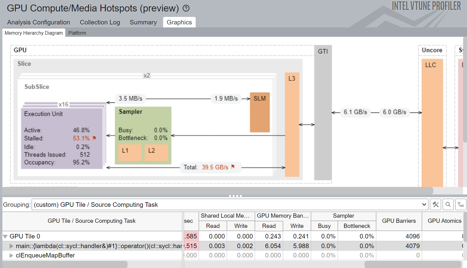
Figure 4. Memory Hierarchy Diagram view of Hierarchical Parallel Kernel Implementation
Figure 4 shows the Memory Hierarchy Diagram and various performance metrics for the Hierarchical Parallel Kernel implementation. This form of kernel implicitly inserts a barrier for every work-group and makes sure the work items communicate through the Shared Local Memory.
As a result, we get a more balanced GTI read and write bandwidth of 6.1 GB/s and 6 GB/s respectively.
It also shows a L3 Bandwidth of 39.5 GB/s which is significantly higher than the ND_Range Kernel implementation.
We achieved ever higher thread occupancy, and thus better overall performance, applying these 3 SYCL kernels for heterogenous compute.
Next, we will look at ways to efficiently tailor data-handling on a heterogenous compute setup using SYCL. Beyond minimizing data transfer across compute units, how can we best manage data exchange between host (CPU) and target (GPU)?
Managing Memory and Data Using SYCL Features
Transferring data to the device, managing device and host memory, and sending data back to the host play a very significant role in heterogeneous programming.
In SYCL, these operations can be performed either explicitly (by application) or implicitly (through runtime) based on the programmer’s requirements and implementation.
Here we discuss 3 different SYCL memory and data management techniques:
1. Buffer-Accessor
A buffer is an encapsulation of data that can allocate memory regions of the host or offload-target device during runtime. However, for conveniently accessing buffers for reading or writing data, the help of accessors is required.
The buffer::get_access(handler&) method consists of two template parameters.
The first is the access mode which can be read, write, read_write, discard_write, discard_read_write, and atomic.
The second parameter is the memory type used by the accessor.
The code segment below illustrates buffer-accessor usage:
buffer<int,2> buff(range<2>(N,M));
device_queue.submit([&](handler &h){
    auto buffer_accessor_device = buff.get_access<access::mode::write>(h);
    /****Kernel****/
});
auto buffer_accessor_host = buff.get_access<access::mode::read>();
Once we run GPU-Offload analysis on the Buffer-Accessor implementation, we get a detailed report of the time spent in various types of operations. The analysis also provides us with recommendations on other analyses or actions needed.
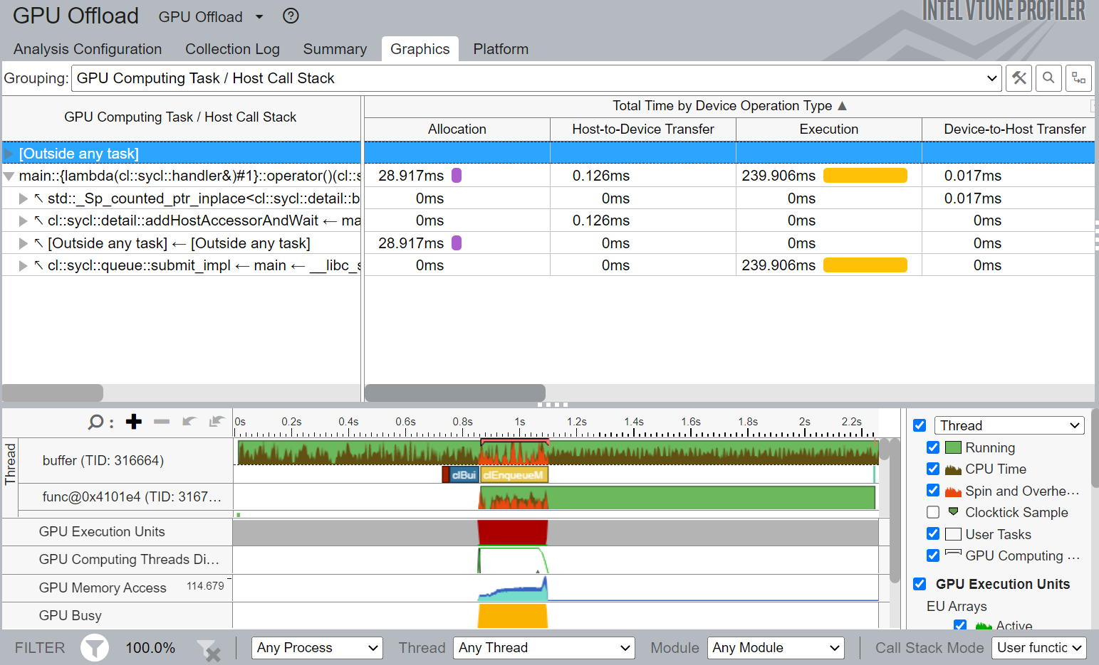
Figure 5. Graphics view of Buffer-Accessor Implementation
Figure 5 shows the Graphics view of Buffer-Accessor Implementation. It shows that it took the SYCL runtime 28.917 ms to allocate memory on the device. It also shows that it takes 0.126 and 0.017 ms to transfer data from host to device and device to host respectively. Total execution time for the kernel is 239.6 ms.
This is our performance characterization baseline.
2. Implicit Unified Shared Memory
The use of implicit Unified Shared Memory (USM) offers an automatic data-movement technique where the programmer does not have to explicitly write the copy operation.
In this case, both host-to-device and device-to-host data transfers are maintained by SYCL runtime. The malloc_shared template function is used for allocating shared memory, which can be accessed by both the host and device. This function takes 1 template parameter and multiple function parameters.
auto **array_shared = malloc_shared<int*>(N, device_queue);
for(int i=0;i<N;i++) {
    array_shared[i] = malloc_shared<int>(M, device_queue);
}
device_queue.submit([&](handler &h){
	/****Kernel****/

}).wait();
3. Explicit Unified Shared Memory
This technique allows programmers to explicitly control the data movement from host to device and device to host using device allocation API calls and a memcpy() function included in the handler class.
The malloc_device function used for allocating device memory takes the size of the 2d array and queue used for execution as parameters. For the memcpy function, the parameters are the device array, host array, and the size of data to be transferred.
auto *array_device = malloc_device<int>(N*M, device_queue);
auto *array_host = malloc_host<int>(N*M, device_queue);
device_queue.submit([&](handler& h) {
    h.memcpy(array_device, &array_host[0], N*M* sizeof(int));
}).wait();
device_queue.submit([&](handler &h){
            /****Kernel****/
    });
}).wait();
Alternatively, we can use sycl::malloc_device to create an array of pointers on the device and use memset or fill (member of the handler and queue classes) function to initialize the 2d array on the device:
auto **array_device = malloc_device<int*>(N, defaultqueue);
auto **array_host = malloc_host<int*>(N, defaultqueue);
for(int i=0;i<N;i++) {
    array_host[i] = malloc_host<int>(M, defaultqueue);
}
defaultqueue.memset(array_device, 0, N*M*sizeof (array_device)).wait();
defaultqueue.submit([&](handler& h) {
    h.memcpy(array_device, &array_host[0], N*M* sizeof(int));
}).wait();

defaultqueue.submit([&](handler &h){
    /*** Kernel ***/
}).wait();
defaultqueue.submit([&](handler& h) {
    h.memcpy(array_host, &array_device[0], (N*M)*sizeof(int));
}).wait();

Figure 6. Graphics view of Explicit Unified Shared Memory Implementation
Figure 6 again shows the VTune Profiler Graphics view of the USM Implementation. It shows the breakdown of total time by device operation type (memory allocation in device, data transfer, execution).
How you manage data transfer in your heterogeneous system is central to workload performance.
Summary
You have seen how you can use SYCL’s powerful yet easy-to-use kernel and memory management techniques to extend serial C++ code to parallel cross-architecture SYCL code. You have also seen how you can leverage Intel VTune Profiler’s GPU insights and interpret its analysis to inform performance-optimization steps.
Additional Resources
To find out more about the Intel® oneAPI Toolkits and the Intel oneAPI DPC++/C++ Compiler as well as the Intel VTune Profiler, please check out the following documents:
- Essentials of SYCL
- Data Parallel C++
- Get Started with the Intel oneAPI DPC++/C++ Compiler
- Intel oneAPI DPC++/C++ Compiler Developer Guide and Reference
- Intel VTune Profiler User Guide
- oneAPI Training Catalog
Get the Software
Download Intel VTune Profiler and Intel oneAPI DPC++/C++ Compiler standalone or as part of the Intel® oneAPI Base Toolkit, a core set of tools and libraries for developing performant, data-centric applications across CPUs, GPUs, FPGAs, and other accelerators.