The original article is published by Intel Game Dev on VentureBeat*: An introduction to neural networks with an application to games. Get more game dev news and related topics from Intel on VentureBeat.
By: Dean Macri
Introduction
Speech recognition, handwriting recognition, face recognition: just a few of the many tasks that we as humans are able to quickly solve but which present an ever increasing challenge to computer programs. We seem to be able to effortlessly perform tasks that are in some cases impossible for even the most sophisticated computer programs to solve. The obvious question that arises is "What's the difference between computers and us?".
We aren't going to fully answer that question, but we are going to take an introductory look at one aspect of it. In short, the biological structure of the human brain forms a massive parallel network of simple computation units that have been trained to solve these problems quickly. This network, when simulated on a computer, is called an artificial neural network or neural net for short.
Figure 1 shows a screen capture from a simple game that I put together to investigate the concept. The idea is simple: there are two players each with a paddle, and a ball that bounces back and forth between them. Each player tries to position his or her paddle to bounce the ball back towards the other player. I used a neural net to control the movement of the paddles and through training (we'll cover this later) taught the neural nets to play the game well (perfectly to be exact).
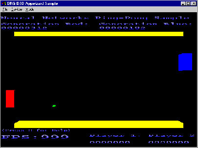
Figure 1: Simple Ping-pong Game for Experimentation
In this article, I'll cover the theory behind one subset of the vast field of neural nets: back-propagation networks. I'll cover the basics and the implementation of the game just described. Finally, I'll describe some other areas where neural nets can be used to solve difficult problems. We'll begin by taking a simplistic look at how neurons work in your brain and mine.
Neural Network Basics
Neurons in the Brain
Shortly after the turn of the 20th century, the Spanish anatomist Ramón y Cajál introduced the idea of neurons as components that make up the workings of the human brain. Later, work by others added details about axons, or output connections between neurons, and about dendrites, which are the receptive inputs to a neuron as seen in Figure 2.
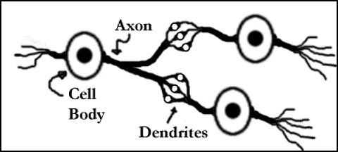
Figure 2: Simplified Representation of a Real Neuron
Put simplistically, a neuron functionally takes many inputs and combines them to either produce an excitatory or inhibitory output in the form of a small voltage pulse. The output is then transmitted along the axon to many inputs (potentially tens of thousands) of other neurons. With approximately 1010neurons and 6×10¹³ connections in the human brain¹ it's no wonder that we're able to perform the complex processes we do. In nervous systems, massive parallel processi ng compensates for the slow (millisecond+) speed of the processing elements (neurons).
In the remainder of this article, we'll cover how artificial neurons, based on the model just described, can be used to mimic behaviors common to humans and other animals. While we can't simulate 10 billion neurons with 60 trillion connections, we can give you a simple worthy opponent to enrich your game play.
Artificial Neurons
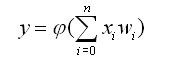
Using the simple model just discussed, researchers in the middle of the 20th century derived mathematical models for simulating the workings of neurons within the brain. They chose to ignore several aspects of real neurons such as their pulse-rate decay and came up with an easy-to-understand model. As illustrated in Figure 3, a neuron is depicted as a computation block that takes inputs (X0, X1Xn) and weights (W0, W1 Wn), multiplies them and sums the results to produce an induced local field, v, which then passes through a decision function, φ(v), to produce a final output, y.
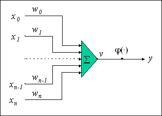
Figure 3: Mathematical model of a neuron
Put in the form of a mathematical equation, this reduces to:
I introduced two new terms, induced local field and decision function, while describing the components of this model so let's take a look at what these mean. The induced local field of a neuron is the output of the summation unit, as indicated in the diagram. If we know that the inputs and the weights can have values that range from -? to +?, then the range of the induced local field is the same. If just the induced local field was propagated to other neurons, then a neural network could perform only simple, linear calculations. To enable more complex computation, the idea of a decision function was introduced. McCulloch and Pitts introduced one of the simplest decision functions in 1943. Their function is just a threshold function that outputs one if the induced local field is greater than or equal to zero and outputs zero otherwise. While some simple problems can be solved using the McCulloch-Pitts model, more complex problems require a more complex decision function. Perhaps the most widely used decision function is the sigmoid function given by:
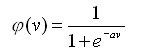
The sigmoid function has two important properties that make it well-suited for use as a decision function:
- It is everywhere differentiable (unlike the threshold function), which enables an easy way to train networks, as we'll see later.
- Its output includes ranges that exhibit both nonlinear and linear behavior.
Other decision functions like the hyperbolic tangent ?(v)=tanh(v), are sometimes used as well. For the examples we'll cover, we'll use the sigmoid decision function unless otherwise noted.
Connecting the Neurons
We've covered the basic building blocks of neural networks with our look at the mathematical model of an artificial neuron. A single neuron can be used to solve some relatively simple problems, but for more complex problems we have to examine a network of neurons, hence the term: neural network.
A neural network consists of one or more neurons connected into one or more layers. For most networks, a layer contains neurons that are not connected to one another in any fashion. While the interconnect pattern between layers of the network (its "topology") may be regular, the weights associated with the various inter-neuron links may vary drastically. Figure 4 shows a three-layer network with two nodes in the first layer, three nodes in the second layer, and one node in the third layer. The first-layer nodes are called input nodes, the third-layer node is called an output node, and nodes in the layers in between the input and output layers are called hidden nodes.
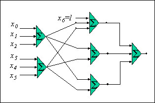
Figure 4: A Three-Layer Neural Network
Notice the input labeled, x6, on the first node in the hidden layer. The fixed input (x6) is not driven by any other neurons, but is labeled as being a constant value of one. This is referred to as a bias and is used to adjust the firing characteristics of the neuron. It has a weight (not shown) associated with it, but the input value will never change. Any neuron can have a bias added by fixing one of its inputs to a constant value of one. We haven't covered the training of a network yet, but when we do, we'll see that the weight affecting a bias can be trained just like the weights of any other input.
The neural networks we'll be dealing with will be structurally similar to the one in Figure 4. A few key features of this type of network are:
- The network consists of several layers. There is one input layer and one output layer with zero or more hidden layers
- The network is not recurrent which means that the outputs from any node only feed inputs of a following layer, not the same or any previous layer.
- Although the network shown in Figure 4 is fully connected, it is not necessary for every neuron in one layer to feed every neuron in the following layer.
Neural Networks for Computation
Now that we've taken a brief look at the structure of a neural network, let's take a quick look at how computation can be performed using a neural network. Later in the paper we'll learn how to go about adjusting weights or training a network to perform a desired computation.
At the simplest level, a single neuron produces one output for a given set of inputs and the output is always the same for that set of inputs. In mathematics, this is known as a function or mapping. For that neuron, the exact relationship between inputs and outputs is given by the weights affecting the inputs and by the particular decision function used by the neuron.
Let's look at a simple example that's common ly used to illustrate the computational power of neural networks. For this example, we will assume that the decision function used is the McCulloch-Pitts threshold function. We want to examine how a neural network can be used to compute the truth table for an AND logic gate. Recall that the output of an AND gate is one if both inputs are one and zero otherwise. Figure 5 shows the truth table for the AND operator.
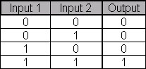
Figure 5: Truth Table for AND Operator
We want to construct a neural network that has two inputs, one output, and calculates the truth table given in Figure 5.
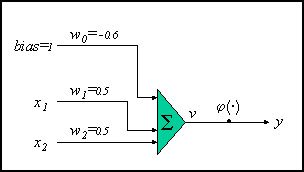
Figure 6: Neuron for Computing an AND Operation
Figure 6 shows a possible configuration of a neuron that does what we want. The decision function is the McCulloch-Pitts threshold function mentioned previously. Notice that the bias weight (w0) is -0.6. This means that if both X1 and X2 are zero then the induced local field, v, will be -0.6 resulting in a 0 for the output. If either X1 or X2 is one, then the induced local field will be 0.5+(-0.6)= -0.1 which is still negative resulting in a zero output from the decision function. Only when both inputs are one will the induced local field go non-negative (0.4) resulting in a one output from the decision function.
While this use of a neural network is overkill for the problem and has a fairly trivial solution, it's the start of illustrating an important point about the computational abilities of a single neuron. We're going to examine this problem and another one to understand the concept of linearly separable problems.
Look at the "graph" in Figure 7. Here, the x-axis corresponds to input 0 and the y-axis corresponds to input 1. The outputs are written into the graph and correspond to the truth table from Figure 5. The gray shaded area represents the region of values that produce a one as output (if we assume the inputs are valid along the real line from zero to one).
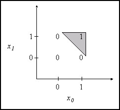
Figure 7: Graph of an AND Function
The key thing to note is that there is a line (the lower left slope of the gray triangle) that separates input values that yield an output of one from input values that yield an output of zero. Problems for which such a "dividing line" can be drawn (such as the AND problem), are classified as linearly separable problems.
Now let's look at another Boolean operation, the exclusive-or (XOR) operation as given in Figure 8.
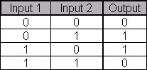
Figure 8: Truth Table for the XOR Operator
Here, the output is one only if one, but not both, of the inputs is one. The "graph" of this operator is shown in Figure 9.
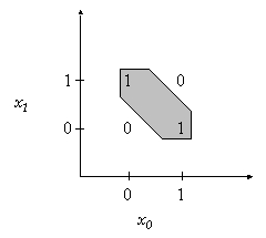
Figure 9: Graph of an XOR Function
Notice that the gray region surrounding the "one" outputs is separated from the zero outputs by not one line, but two lines (the lower and upper sloping lines of the gray region). This problem is not linearly separable. If we try to construct a single neuron that can calculate this function, we won't succeed.
Early researchers thought that this was a limitation of all computation using artificial neurons. It is only with the addition of multiple layers that it was realized that neurons that were linear in behavior could be combined to solve problems that were not linearly separable. Figure 10 shows a simple, three-neuron network that can solve the XOR problem. We're still assuming that the decision function is the McCulloch-Pitts threshold function.
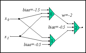
Figure 10: Network for Calculating XOR Function
All the weights are fixed at 1.0 with the exception of the weight labeled as w=-2. For completeness, let's quickly walk through the outputs for the four different input combinations.
- If both inputs are 0, then neurons 0 and 1 both output 0 (because of their negative biases). Thus, the output of neuron 2 is also 0 due to its negative bias and zero inputs.
- If X0 is 1 and X1 is 0, then neuron 0 outputs 0, neuron 1 outputs 1 (because 1.0+(-0.5)=0.5 is greater than 0) and neuron 2 then outputs a 1 also.
- If X0 is 0 and X1 is 1, then neuron 0 outputs 0, neuron 1 outputs 1, and neuron 2 outputs 1.
- Finally, if both inputs are 1, then neuron 0 outputs a 1 that becomes a -2 input to neuron 2 (because of the negative weight). Neuron 1 outputs a 1 which combines with -2 and the -0.5 bias to produce an output of 0 from neuron 2.
The takeaway from this simple example is that to solve non-linearly separable problems, multi-layer networks are needed. In addition, while the McCulloch-Pitts threshold function works fine for these easy to solve problems, a more mathematically friendly (i.e. differentiable) decision function is needed to solve most real world problems. We'll now get into the way a neural network can be trained (rather than being programmed or structured) to solve a particular problem.
Learning Processes
Let's go way back to the definition of the output of a single neuron (we've added a parameter for a particular set of data, k):
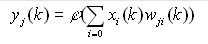
Equation 1
Note here that x = y, the output from neuron i, if neuron j is not an input neuron. Also, w is the weight connecting output of neuron i as an input to neuron j.
We want to determine how to change the values of the various weights, w(k), when the output, y(k), doesn't agree with the result we expect or require from a given set of inputs, x(k). Formally , let d(k) be the desired output for a given set of inputs, k. Then, we can look at the error function, e(k)=d(k)-y(k). We want to modify the weights to reduce the error (ideally to zero). We can look at the error energy as a function of the error:
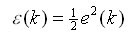
Equation 2
Adjusting the weights now becomes a problem of minimizing ?(k). We want to look at the gradient of the error energy with respect to the various weights,

. Combining Equation 1 and Equation 2 and using the chain rule (and recalling that y(k)=?(v(k)) and v(k)=?w(n)y(n) ), we can expand this derivative to something more manageable:
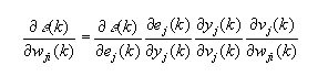
Equation 3
Each of the terms in Equation 3 can be reduced so we get:
Equation 4
Where ?'() signifies differentiation with respect to the argument. Adjustments to the weights can be written using the delta rule:
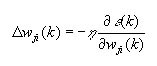
Equation 5
Here, ? is a learning-rate parameter that varies from 0 to 1. It determines the rate at which weights are changed to move "up the gradient". If ? is 0, no learning will take place. We can re-write Equation 5 to include what is known as the local gradient, ?(k):
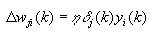
Equation 6
Here,
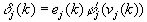
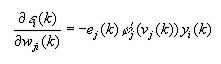
Equation 6 can be used directly to update the weights of a neuron in the output layer of a neural network. For neurons in hidden and inputs layers of a network, the calculations are slightly more complex. To calculate the weight changes for these neurons, we use what is known as the back-propagation formula. I won't go through the details of the derivation, but the formula for the local gradient reduces to:
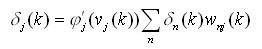
Equation 7
In this formula, w(k) represents the weights connecting the output of neuron, j, to an input of neuron n. Once we've calculated the local gradient, ?j, for this neuron, we can use Equation 6 to calculate the weig ht changes.
To compute the weight changes for all the neurons in a network, we start with the output layer. Using Equation 6 we first compute the weight changes for all the neurons in the output layer of the network. Then, using Equation 6 and Equation 7 we compute the weight changes for the hidden layer closest to the output layer. We use these equations again for each additional hidden layer working from outputs toward inputs and from right to left, until weight changes for all the neurons in the network have been calculated. Finally we apply the weight changes to the weights, at which point we can recompute the network output to see if we've gotten closer to the desired result.
Network training can occur in several different ways:
- The weight changes can be accumulated over several input patterns and then applied after all input patterns have been presented to the network.
- The weight changes can be applied to the network after each input pattern is presented.
Method 1 is most commonly used. When method 2 is used, the patterns are presented to the network in a random order. This is necessary to keep the network from possibly becoming "trapped" in some presentation-order-sensitive local energy minimum.
Before looking at an example problem, let me wrap up this section by noting that I've only discussed one type of learning process: back-propagation using error-correction learning. Other types of learning processes include memory-based learning, Hebbian learning and competitive learning. Refer to the references at the end of this article for more information on these techniques.
Putting Neural Nets to Work
Let's take a closer look at the game I described in the introduction. Figure 11 shows a screen capture of the game after several generations of training.
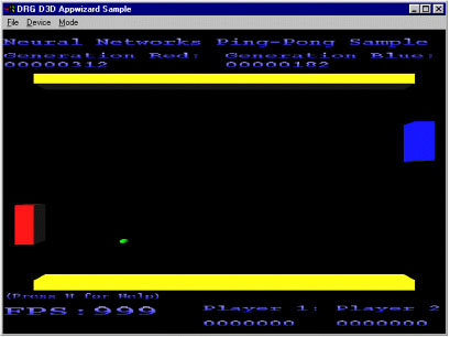
Figure 11: Ping-Pong Sample Application
The training occurs by shooting the ball from the center with a random direction (the speed is fixed). The neural network is given as input the (x,y) position of the ball as well as the direction and the y position of the paddle (either red or blue depending upon which paddle the ball is heading towards). The network is trained to output a y direction that the paddle should move.
I created a three-layered network with three nodes in the input layer, ten nodes in the hidden layer, and one node in the output layer. The input nodes each get the same five inputs corresponding to the (x,y) position and direction of the ball and the y position of the paddle. These nodes are fully connected to the nodes in the hidden layer, which are in turn fully connected to the output node. Figure 12 shows the layout of the network with inputs and outputs. Weights, biases, and decision functions are not shown.
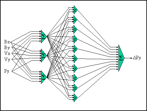
Figure 12: Neural Network for Ping Pong Game
The network learns to move the paddle in the same y-direction that the ball is heading. After several thousand generations of training, the neural network learns to play perfectly (the exact number of generations varies because the network weights are initialized to random values).
I experimented with using a paddle speed that was slower than the speed of the ball so that the networks would have to do some form of prediction. With the network from Figure 12 some learning took place but the neural nets weren't able to learn to play perfectly. Some additional features would have to be added to the network to enable it to fully learn this problem.
In this example, the neural network is the only form of AI that the computer controlled opponent has. By varying the level of training, the computer opponent can vary from poor play to perfect play. Deciding when to stop the training is a non-trivial challenge. One easy solution would be to train the network for some number of iterations up front (say 1000) and then each time the human player wins, train the network an additional 100 iterations. Eventually this would produce a perfect computer-controlled opponent, but should also produce a progressively more challenging opponent.
Non-trivial Applications of Neural Nets
While the ping-pong example provides an easy to understand application of neural nets to artificial intelligence, real-world problems require a bit more thought. I'll briefly mention a few possible uses of neural nets, but realize that there isn't going to be a one-size-fits-all neural network that you can just plug into your application and solve all your problems. Good solutions to specific problems require considerable thought and experimentation with what variables or "features" to use as network input and outputs, what size and organization of network to use, and what training sets are used to train the network.
Using a neural network for the complete AI in a game probably isn't going to work well for anything beyond the simple ping-pong example previously discussed. More likely than not, you're going to use a traditional state machine for the majority of AI decisions but you may be able to use neural nets to complement the decisions or to enhance the hard-coded state machine. An example of this might be a neural net that takes as input such things as health of the character, available ammunition, and perhaps health and ammunition of the human opponent. Then, the network could decide whether to fight or flee at which point the traditional AI would take over to do the actual movement, path-finding, etc. Over several games, the network could improve its decision making process by examining whether each decision produced a win or a loss (or maybe less globally, an increase or decrease in health and/or ammunition).
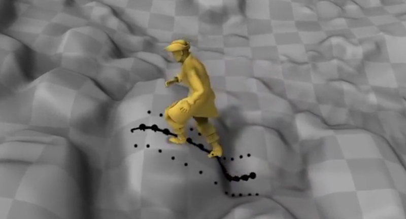
One area that intrigues me and which has had some research devoted to it is the idea of using neural networks to perform the actual physics calculations in a simulation². I think this has promise because training a neural network is ultimately a process of finding a function that fits several sets of data. Given the challenge of creating physical controllers for physically simulated games, I think neural networks are one possibility for solutions there as well.
The use of neural nets for pattern recognition of vario us forms is their ultimate strength. Even in the problems described, the nets would be used for recognizing patterns, whether health and ammunition, forces acting on an object, or something else, and then take an appropriate action. The strength lies in the ability of the neural nets to be trained on a set of well-known patterns and then be able to extract meaningful decisions when presented with unknown patterns. This feature of extrapolation from existing data to new data can be applied to the areas of speech recognition, handwriting recognition and face recognition mentioned in the introduction. And it can also be beneficial to "fuzzy" areas like finding trends in stock market analysis.
Conclusion
I've tried to keep the heavy math to a minimum, the details about sample code pretty much out of the picture, and still provide a solid overview of back-propagation neural networks. Hopefully this article has provided a simple overview of neural networks and given you some simple sample code to examine to see if neural networks might be worth investigating for decision-making in your applications. I'd recommend checking out some of the references to gain a more solid understanding of all the quirks of neural networks. I encourage you to experiment with neural networks and come up with novel ways in which they can add realism to upcoming game titles or enhance your productivity applications.