Using Fast Fourier Transforms for computer tomography image reconstruction
Goal
Reconstruct the original image from the Computer Tomography (CT) data using fast Fourier transform (FFT) functions.
Solution
Notation:
Specification of index ranges adopts the notation used in MATLAB*.
For example: k=-q : q means k=-q, -q+1, -q+2,…, q-1, q.
While f(x) means the value of the function f at point x, f[n] means the value of nth element of the discrete data set f.
Assumptions:
The density f(x, y) of a two-dimensional (2D) image vanishes outside the unit circle:
f = 0 when x2 + y2 > 1.
The CT data consists of p projections of the image taken at angles θj = jπ/p, where j = 0 : p - 1.
Each projection contains 2q + 1 density values g[j, l] = g(θj , sl) approximating the integral of the image along the line
(x, y) = (-t sinθj+ sl cosθj , t cosθj+ sl sinθj),
where l = -q : q, sl= l /q, and t is the integration parameter.
The discrete image reconstruction algorithm consists of the following steps:
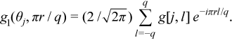
Evaluate p one-dimensional (1D) Fourier transforms (for j = 0 : p - 1 and r = -q : q):
Interpolate g1[j, r] from radial grid (πr/q)(cosθj , sinθj) onto Cartesian grid (ξ, η) = (-q : q, -q : q), obtaining f2(πξ/q, πη/q).
Evaluate one inverse two-dimensional complex-to-complex FFT to obtain a complex-valued reconstruction f1 of the image:
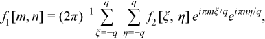
where f(m/q, n/q) ≈f1[m, n] for m = -q : q and n = -q : q.
Computations in steps 1 and 3 call oneMKL FFT interfaces. Computations in step 2 implement a simple version of interpolation tailored to the data layout used by oneMKL FFT.
Reconstructing the original CT image in C/C++
// Declarations
int Nq = 2*(q+1); // space for in-place r2c FFT
void    *gmem = mkl_malloc( sizeof(float)*p*Nq, 64 );
float    *g = gmem; // g[j*Nq + ell+q]
complex *g1 = gmem; // g1[j*Nq/2 + r+q]

// Initialize g with the CT data
for (int j = 0; j < p; ++j)
for (int ell = 0; ell < 2*q+1; ++ell) {
  g[j*Nq + ell+q] = get_g(theta_j,s_ell);
}

// Step 1: Configure and compute 1D real-to-complex FFTs
DFTI_DESCRIPTOR_HANDLE h1 = NULL;
DftiCreateDescriptor(&h1,DFTI_SINGLE,DFTI_REAL,1,(MKL_LONG)2*q);
DftiSetValue(h1,DFTI_CONJUGATE_EVEN_STORAGE,DFTI_COMPLEX_COMPLEX);
DftiSetValue(h1,DFTI_NUMBER_OF_TRANSFORMS,(MKL_LONG)p);
DftiSetValue(h1,DFTI_INPUT_DISTANCE,(MKL_LONG)Nq);
DftiSetValue(h1,DFTI_OUTPUT_DISTANCE,(MKL_LONG)Nq/2);
DftiSetValue(h1,DFTI_FORWARD_SCALE,fscale);
DftiCommitDescriptor(h1);
DftiComputeForward(h1,g); // now gmem contains g1

// Step 2: Interpolate g1 to f2 - omitted here
complex *f = mkl_malloc( sizeof(complex) * 2*q * 2*q, 64 );

// Step 3: Configure and compute 2D complex-to-complex FFT
DFTI_DESCRIPTOR_HANDLE h3 = NULL;
MKL_LONG sizes[2] = {2*q, 2*q};
DftiCreateDescriptor(&h3,DFTI_SINGLE,DFTI_COMPLEX,2,sizes);
DftiCommitDescriptor(h3);
DftiComputeBackward(h3,f); // now f is complex-valued reconstruction
Source code, image file, and makefiles: see the fft-ct folder in the samples archive available at https://www.intel.com/content/dam/develop/external/us/en/documents/mkl-cookbook-samples-120115.zip.
Discussion
The code first configures the oneMKL FFT descriptor for computing a batch of the one-dimensional Fourier transforms in a single call to the DftiComputeForward function and then computes the batch transform. The distance for the multiple transforms is set in terms of elements of the corresponding domain (real on input and complex on output). The transforms are in-place by default.
To have a smaller memory footprint, the FFT is computed in place, that is, the result of the computation overwrites the input data. With an in-place real-to-complex FFT the input array reserves extra space because the result of the FFT takes slightly more memory than the input.
On input to step 1, array g contains p x (2q+1) real-valued data elements g(θj, sl). The same memory on output of this step contains p x (q + 1) complex-valued output elements g1(θj, πr/q). The complex-conjugate part of the result is not stored, and therefore array g1 refers to only q + 1 values of r.
To interpolate from g1 to f2, an additional array f is allocated to store complex-valued data f2(ξ, η) and complex-valued output f1(x, y) of inverse FFT in step 3. The interpolation step does not call oneMKL functions, but you can find its C++ implementation in the function step2_interpolation of the source code for this recipe (file main.cpp). The simplest implementation of interpolation is:
For every (ξ, η) inside the unit circle, find the closest (θj , πr/q) and use the value of g1(θj , πr/q) for f2.
- For every (ξ, η) outside the unit circle, set f2 to 0.
In the case of (ξ, η) corresponding to the interval -π < θj < 0, use conjugate even property of the result of a real-to-complex transform: g1(θ, ω)=conj(g(-θ, -ω)).
Notice that the FFT in step 1 is applied to the data offset by half the representation interval, which causes the computed output be multiplied by ei(πr/q)q= (-1)r. Instead of correcting this in a separate pass, the interpolation takes the multiplier into account.
Similarly, the 2D FFT in step 3 produces an output that shifts the center of the image to the corner, and step 2 prevents this by phase shifting the input to step 3.
Step 3 computes the two-dimensional (2q) x (2q) complex-to-complex FFT on the interpolated data contained in array f. This computation is followed by a conversion of the complex-valued image f1 to a visual picture. You can find a complete C++ program that implements the CT image reconstruction in the source code for this recipe (file main.cpp).
Parent topic: Intel® oneAPI Math Kernel Library Cookbook